You are here: Experiment Guide > Imaging Modes > Force Spectroscopy > Nanomechanical Property Mapping

Nanomechanical Property Mapping

The mechanical mapping function in force volume lets you fit various indentation models to measured force curves and compute the sample modulus and adhesion.

Models

Several indentation models are available:

Hertz model (spherical indenter)

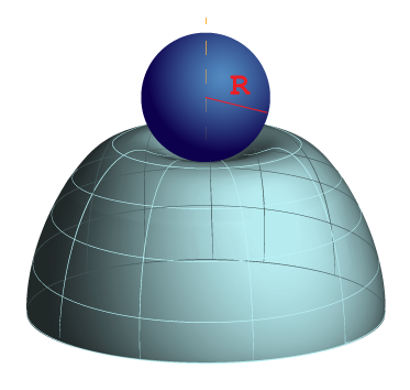
Figure 1: Contact between a sphere and an elastic half-space

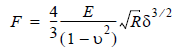
Equation 2: Hertzian model

where

F = force (from force curve)

E = Young's modulus (fit parameter)

ν = Poisson's ratio (sample dependent, typically 0.2 - 0.5)

R = radius of the indenter (tip)

δ = indentation

Equation 2 may be linearized in separation by taking both sides to the 2/3 power, shown in Equation 3.

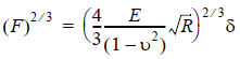
Equation 3: Linearized Hertz equation

Sneddon (conical indenter)

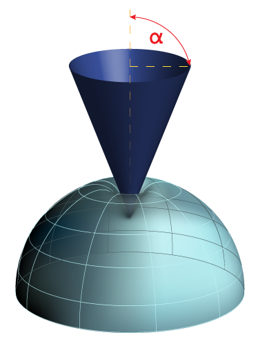
Figure 4: Contact between a cone and an elastic half-space

Equation 5: Sneddon model

where

F = force (from force curve)

E = Young's modulus (fit parameter)

ν = Poisson's ratio (sample dependent, typically 0.2 - 0.5)

α = half-angle of the indenter

δ = indentation

Equation 5 may be linearized in separation by taking both sides to the 1/2 power, shown in Equation 6.

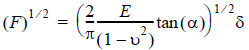
Equation 6: Linearized Sneddon equation

Depending on the model, Young's modulus is computed from the slope of either Equation 3 or Equation 6.

Stiffness (linear)

The stiffness model extrapolates a straight line fit to the maximum indentation.

Nanomechanical Property Mapping Procedure

If you are using the Hertzian model, enter the probe Tip Radius .
If you are using the Sneddon model, enter the probe Tip Half Angle.
Enter the Sample's Poisson Ratio.
Decide if you wish to Include Adhesion Force.

Including Adhesion Force means that calculations are performed based on forces relative to the adhesion force. Otherwise, calculations are performed on absolute force values.

Enter a value for the Minimum Force Fit Boundary. The Minimum Force Fit Boundary is defined as a percentage of the [(Maximum Force) - (Minimum Force)]. See Figure 7.
Enter a value for the Maximum Force Fit Boundary. The Maxmimum Force Fit Boundary is defined as a percentage of the [(Maximum Force) - (Minimum Force)].

These boundaries define the region through which the fit model is computed.

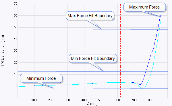
Figure 7: Minimum and Maximum Force Fit Boundaries defined

Select a Modulus Fit Model:

Hertz model (spherical indenter)
Sneddon (conical indenter)

Select the Z direction that you wish to use for the Modulus Fit Model: Extend or Retract.

NOTE: You choice of Z direction here also determines which portion of the Real-time force curve cycle, Extend or Retract, is shown in the force volume image.

Enter the Spring Constant.
Select the display properties of the two force volume images:

Data Type:

Deflection Error
FV Modulus: Maps the modulus using the selected Modulus Fit Model.
FV Log Modulus: Maps the log of the modulus using the selected Modulus Fit Model.
FV Adhesion: The peak force below the baseline. See Figure 8.

Figure 8: Adhesion

NOTE: 1st order baseline correction, which removes baseline tilt as well as offset, is performed before adhesion mapping.

FV Stiffness: Maps the Stiffness (linear).

Data Center: Refer to Detailed Force Volume Procedure for details.
Data Scale: Refer to Detailed Force Volume Procedure for details.
Z display: Used only when Data Type is Deflection Error. Refer to Detailed Force Volume Procedure for details.

www.bruker.com	Bruker Corporation
www.brukerafmprobes.com	112 Robin Hill Rd.
nanoscaleworld.bruker-axs.com/nanoscaleworld/	Santa Barbara, CA 93117

	Customer Support: (800) 873-9750
	Copyright 2010, 2011. All Rights Reserved.